Google Data Analytics Capstone Project - BellaBeat

Table of Contents
Introduction #
This is the case study that served as my capstone project for Google’s Data Analytics Course. I aimed to use as many of the skills I learned in that course while completing this project, including spreadsheets, SQL, and RStudio. I chose this case study in particular for it’s focuse on exercise and physical fitness, topics that I have a deep interest in. Beyond the Data Analytics Certificate, I hope that this project will help me learn how to better use my own Fitbit data.
Prompt #
You are a junior data analyst working on the marketing analyst team at Bellabeat, a high-tech manufacturer of health-focused products for women. Bellabeat is a successful small company, but they have the potential to become a larger player in the global smart device market. Urška Sršen, cofounder and Chief Creative Officer of Bellabeat, believes that analyzing smart device fitness data could help unlock new growth opportunities for the company. You have been asked to focus on one of Bellabeat’s products and analyze smart device data to gain insight into how consumers are using their smart devices. The insights you discover will then help guide marketing strategy for the company. You will present your analysis to the Bellabeat executive team along with your high-level recommendations for Bellabeat’s marketing strategy
Urška Sršen and Sando Mur founded Bellabeat, a high-tech company that manufactures health-focused smart products. Sršen used her background as an artist to develop beautifully designed technology that informs and inspires women around the world. Collecting data on activity, sleep, stress, and reproductive health has allowed Bellabeat to empower women with knowledge about their own health and habits. Since it was founded in 2013, Bellabeat has grown rapidly and quickly positioned itself as a tech-driven wellness company for women.
By 2016, Bellabeat had opened offices around the world and launched multiple products. Bellabeat products became available through a growing number of online retailers in addition to their own e-commerce channel on their website. The company has invested in traditional advertising media, such as radio, out-of-home billboards, print, and television, but focuses on digital marketing extensively. Bellabeat invests year-round in Google Search, maintaining active Facebook and Instagram pages, and consistently engages consumers on Twitter. Additionally, Bellabeat runs video ads on Youtube and display ads on the Google Display Network to support campaigns around key marketing dates.
Sršen knows that an analysis of Bellabeat’s available consumer data would reveal more opportunities for growth. She has asked the marketing analytics team to focus on a Bellabeat product and analyze smart device usage data in order to gain insight into how people are already using their smart devices. Then, using this information, she would like high-level recommendations for how these trends can inform Bellabeat marketing strategy.
Sršen asks you to analyze smart device usage data in order to gain insight into how consumers use non-Bellabeat smart devices. She then wants you to select one Bellabeat product to apply these insights to in your presentation. These questions will guide your analysis:
- What are some trends in smart device usage?
- How could these trends apply to Bellabeat customers?
- How could these trends help influence Bellabeat marketing strategy?
You will produce a report with the following deliverables:
- A clear summary of the business task:
- A description of all data sources used.
- Documentation of any cleaning or manipulation of data
- A summary of your analysis
- Supporting visualizations and key findings
- Your top high-level content recommendations based on your analysis
Business Task #
We have been tasked to discover trends in device usage, then apply those findings towards helping customers and Bellabeat’s marketing strategy.
Prepare #
The data were collected from thirty-four users who gave informed consent to have their data analyzed. The data have been anonymized. The project wants to evaluate the data on the following criteria:
- Reliable - This data is not very reliable. In addition to the problems listed below, there’s a lack of useful information about the individuals, nor is it clear why these individuals were chosen.
- Original - This data originates from a third party.
- Comprehensive - Only 34 individuals are involved and the data is full of gaps. Some datasets are missing entire days of data.
- Current - This data was gathered in 2016. Granted, health data doesn’t have an exact expiration date and can still be useful years afterward, but one has to wonder why more recent data couldn’t be found, especially since this is supposed to inform the business decisions of a company about to enter a new market.
- Cited - It’s not clear how the Kaggle user who uploaded the data got them in the first place.
Overall, the quality of the data is quite poor. I searched for similar datasets that might make up for these deficiencies, but none were forthcoming even after extensive searching.
Here are a list of the individual datasets along with the columns from each one:
dailyActivity_merged- Id, Activity Date, Total Steps, Total Distance, Tracker Distance, Logged Activities Distance, Very Active Distance, Moderately Active Distance, Lightly Active Distance, Sedentary Active Distance, Very Active Minutes, Fairly Active Minutes, Lightly Active Minutes, Sedentary Minutes, CaloriesdailyCalories_merged- Id, ActivityDay, CaloriesdailyIntensities_merged- Id, Activity Day, Sedentary Minutes, Lightly Active Minutes, Fairly Active Minutes, Very Active Minutes, Sedentary Active Distance, Light Active Distance, Moderately Active Distance, Very Active DistancedailySteps_merged- Id, Activity Day, Step Totalheartrate_seconds_merged- Id, Time, ValuehourlyCalories_merged- Id, Activity Hour, CalorieshourlyIntensities_merged- Id, Activity Hour, Total Intensity, Average IntensityhourlySteps_merged- Id, Activity Hour, Step TotalminuteCaloriesNarrow_merged- Id, Activity Minute, CaloriesminuteCaloriesWide_merged- Id, Activity Hour, Calories per Minute (60)minuteIntensitiesNarrow_merged- Id, Activity Minute, IntensityminuteIntensitiesWide_merged- Id, Activity Hour, Intensity per Minute (60)minuteMETSNarrow_merged- Id, Activity Minute, METsminuteSleep_merged- Id, Date, Value, Log IdminuteStepsNarrow_merged- Id, Activity Minute, StepsminuteStepsWide_merged- Id, Activity Hour, Steps per Minute (60)sleepDay_merged- Id, Sleep Day, Total Sleep Records, Total Minutes Asleep, Total Time In BedweightLogInfo_merged- Id, Date, Weight Kg, Weight Pounds, Fat, BMI, Is Manual Report, Log Id
Most of the data is based on the increments of time in which it was gathered (hourly, daily, etc), so I’ll evaluate and process the data on these terms as well.
Processing #
Daily Data #
The daily data was cleaned and partially processed with Google Sheets. This data comes from the following sets:
dailyActivity_mergeddailyCalories_mergeddailyIntensities_mergeddailySteps_mergedsleepDay_merged
The dailyActivity_merged file is already exhaustive, containing much of the data in the other daily data. As such, the following datasets were removed from the analysis for being redundant: dailyCalories_merged, dailyIntensities_merged, and dailySteps_merged. From this point, it was a simple matter of using Google Sheets to root out duplicate rows and null values, none of which were found.
The only daily data that wasn’t already incorporated in the dailyActivity_merged file was the sleepDay_merged dataset. As an avid fitness enthusiast myself, I know that quality sleep can be just as important as exercise and diet. It seemed obvious to do whatever I could to combine these two datasets in hopes of gaining new insights.
I removed three duplicate rows in the sleepDay_merged dataset. With the COUNTUNIQUE function, I also noticed that there were only 24 unique users in the dataset, as opposed to the 34 in the dailyActivity_merged dataset. I also noticed that users didn’t track their sleep every night. Furthermore, I changed the title of the “value” column to “sleepValue” to clarify its origin.
All told, cleaning the data through Sheets was incredibly simple and I’ll continue using it for some of my analysis.
Finally, I also added the final draft of both spreadsheets to the SQL database to compare it against the rest of the data. Before doing this, I made sure to change the date format so that it would match SQL’s DATE datatype. Using the following SQL query, I was able to merge both datasets together:
SELECT activity.Id, ActivityDate, Calories, sleep.TotalSleepRecords, sleep.TotalMinutesAsleep, sleep.TotalTimeInBed, TotalSteps, TotalDistance, TrackerDistance, LoggedActivitiesDistance, (VeryActiveDistance + ModeratelyActiveDistance) AS ActiveDistance, (LightActiveDistance+SedentaryActiveDistance) AS non_ActiveDistance, (VeryActiveMinutes+FairlyActiveMinutes) AS ActiveMinutes, (LightlyActiveMinutes+SedentaryMinutes) AS non_ActiveMinutes
FROM `Bellabeat.dailyActivity` AS activity
INNER JOIN `Bellabeat.sleepDay` AS sleep
ON activity.Id = sleep.Id AND activity.ActivityDate = sleep.SleepDay
The resulting data was then exported as dailyMerged.csv.
Hourly Data #
The hourly data consists of the following:
hourlyCalories_mergedhourlyIntensities_mergedhourlySteps_merged
This data is too unwieldy to work with in spreadsheets, so these will be processed using tools like R Studio, and SQL. However, Google Sheets was sufficiently capable of carrying out some of the necessary cleaning. Before exporting them from Google Sheets, I checked the data for duplicate rows and reformatted the dates so BigQuery would accept them as DATETIME data type.
I renamed the datasets when I uploaded them to BigQuery to remove the extraneous “_merged” modifier. For example, the minuteSleep_merged dataset became “minuteSleep” and hourlySteps_merged became “hourlySteps”.
Using SQL, I joined the hourly data together with the following query:
SELECT
A.Id,
A. ActivityHour AS activity_hour,
A.Calories,
C.StepTotal AS step_total,
I. TotalIntensity AS total_intensity,
I. AverageIntensity AS average_intensity,

FROM `Bellabeat.hourlyCalories` A

LEFT JOIN `Bellabeat.hourlySteps` C
ON
A.Id = C.Id
AND A.ActivityHour=C.ActivityHour
LEFT JOIN `Bellabeat.hourlyIntensities` I
ON
A.Id = I.Id
AND A.ActivityHour=C.ActivityHour
The resulting data was then exported as hourlyMerged.csv.
Second and Minute Data #
The second and minute data consist of the following:
minuteCaloriesNarrow_mergedminuteCaloriesWide_mergedminuteIntensitiesNarrow_mergedminuteIntensitiesWide_mergedminuteMETSNarrow_mergedminuteSleep_mergedminuteStepsNarrow_mergedminuteStepsWide_mergedheartrate_seconds_merged
These datasets are too unwieldy even for SQL or R. As nice as it is in theory to have everything in fine grained detail, such data need to justify the trouble and strife required to clean, process, and analyze them, which doesn’t appear to be the case with the second and minute data. If there’s no way to aggregate and average this data into more manageable units of time, I’ll have to set it aside for the moment or at least until I have access to more computing power.
Weight Log #
The scant amount of data in weightLogInfo_merged makes this difficult to comfortably incorporate into the study. Only eight of the already paltry thirty-four participants logged their weight, and of those, only two of them did so more than five times. This is especially disappointing considering studies of large populations is one of the few areas where the controversial BMI metric undeniably shines.
Analyze and Visualize #
Daily Data Analysis #
After making a quick few charts in Google Sheets, the sleep tracking data doesn’t appear to correlate strongly with any of the other data, whether that’s calories, steps, or active or sedentary minutes at any intensity. This is disappointing, though unsurprising considering the unreliability and lack of sleep data gathered. Perhaps more insight can be gleaned by using R.
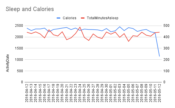
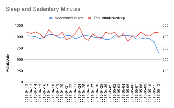
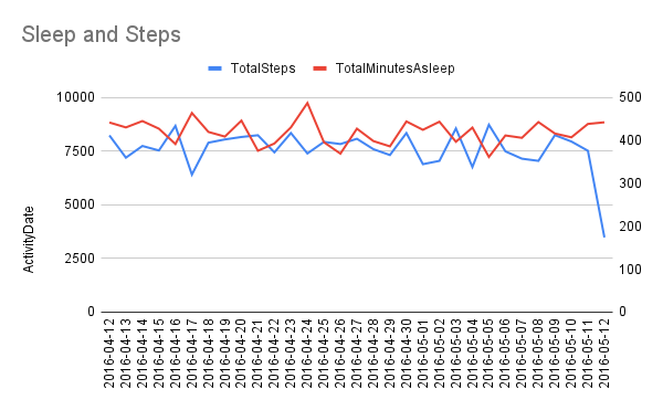
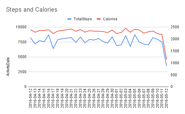
Other charts measuring more banal observations indicate that at least the commonly logged data is internally consistent. For example, the number steps taken each day correlates strongly with calories burned, as does the total distance traveled.
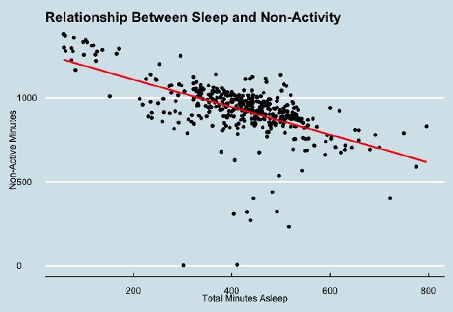
As I’d hoped, I was able to get more insight from bringing the data into RStudio. Although there isn’t a strong correlation between activity and sleep (-0.1815268), it does appear there is a moderate negative correlation between sleep and non-active minutes (-0.5869577). This suggests that sleep has a stronger effect on whether or not an individual will be active the next day:
> library(tidyverse)
> cor.test(dailyMerged1$TotalMinutesAsleep, dailyMerged1$ActiveMinutes, method="pearson")

    Pearson's product-moment correlation

data:  dailyMerged1$TotalMinutesAsleep and dailyMerged1$ActiveMinutes
t = -3.7286, df = 408, p-value = 0.0002197
alternative hypothesis: true correlation is not equal to 0
95 percent confidence interval:
 -0.27356474 -0.08619484
sample estimates:
       cor
-0.1815268

> cor.test(dailyMerged1$TotalMinutesAsleep, dailyMerged1$non_ActiveMinutes, method="pearson")

    Pearson's product-moment correlation

data:  dailyMerged1$TotalMinutesAsleep and dailyMerged1$non_ActiveMinutes
t = -14.644, df = 408, p-value < 2.2e-16
alternative hypothesis: true correlation is not equal to 0
95 percent confidence interval:
 -0.6470247 -0.5196501
sample estimates:
       cor
-0.5869577

>library(ggthemes)
>ggplot(dailyMerged1, aes(x = dailyMerged1$TotalMinutesAsleep, y = dailyMerged1$non_ActiveMinutes))+
  geom_point() + geom_smooth(method=lm, se=FALSE, col="red") + labs(y = "Non-Active Minutes", x = "Total Minutes Asleep") + ggtitle("Relationship Between Sleep and Non-Activity")
With all this daily data, it seemed prudent to aggregate the data by day of the week and see what trends I could find. With the following script, I was able to collate data based on day of the week (this codeblock is very long, so I put most of it behind an expandable section):
> # Monday
>
> day_Monday <- dailyMerged1 %>%
+   filter(dailyMerged1$DayOfWeek == "Monday") %>%
+   select(-c(Id, ActivityDate))
> summary(day_Monday)
    Calories    TotalSleepRecords TotalMinutesAsleep TotalTimeInBed    TotalSteps    TotalDistance
 Min.   :1248   Min.   :1.000     Min.   : 62.0      Min.   : 65.0   Min.   : 1831   Min.   : 1.170
 1st Qu.:1998   1st Qu.:1.000     1st Qu.:368.5      1st Qu.:399.8   1st Qu.: 6937   1st Qu.: 4.787
 Median :2232   Median :1.000     Median :434.0      Median :467.5   Median : 9831   Median : 6.815
 Mean   :2432   Mean   :1.109     Mean   :419.5      Mean   :457.3   Mean   : 9273   Mean   : 6.541
 3rd Qu.:3007   3rd Qu.:1.000     3rd Qu.:492.8      3rd Qu.:528.8   3rd Qu.:11559   3rd Qu.: 8.265
 Max.   :4157   Max.   :2.000     Max.   :796.0      Max.   :961.0   Max.   :16520   Max.   :11.050
 TrackerDistance  LoggedActivitiesDistance ActiveDistance  non_ActiveDistance ActiveMinutes    non_ActiveMinutes
 Min.   : 1.170   Min.   :0.0000           Min.   :0.000   Min.   :1.120      Min.   :  0.00   Min.   : 322.0
 1st Qu.: 4.787   1st Qu.:0.0000           1st Qu.:0.410   1st Qu.:3.045      1st Qu.: 10.25   1st Qu.: 882.5
 Median : 6.815   Median :0.0000           Median :1.975   Median :3.930      Median : 44.50   Median : 931.5
 Mean   : 6.536   Mean   :0.2826           Mean   :2.519   Mean   :4.016      Mean   : 49.80   Mean   : 940.8
 3rd Qu.: 8.265   3rd Qu.:0.0000           3rd Qu.:3.980   3rd Qu.:4.855      3rd Qu.: 77.50   3rd Qu.:1000.0
 Max.   :11.050   Max.   :3.0000           Max.   :8.020   Max.   :6.790      Max.   :167.00   Max.   :1278.0
  DayOfWeek
 Length:46
 Class :character
 Mode  :character

>
> day_Mon_list <-
+   list(
+     list("Total_Steps_Ave" = ~ mean(day_Monday$TotalSteps, na.rm = TRUE)),
+     list("Active_Minutes_Ave" = ~ mean(day_Monday$ActiveMinutes, na.rm = TRUE)),
+     list("Sedentary_Minutes_Ave" = ~ mean(day_Monday$non_ActiveMinutes, na.rm = TRUE)),
+     list("Calories_Ave" = ~ mean(day_Monday$Calories, na.rm = TRUE)),
+     list("Total_Hours_Asleep_Ave" = ~ mean(day_Monday$TotalMinutesAsleep/60, na.rm = TRUE))
+   )
> day_Mon_summary <- summary_table(day_Monday, day_Mon_list)
> print.default(day_Mon_summary)
                       day_Monday (N = 46)
Total_Steps_Ave                9273.217391
Active_Minutes_Ave               49.804348
Sedentary_Minutes_Ave           940.782609
Calories_Ave                   2431.978261
Total_Hours_Asleep_Ave            6.991667
attr(,"rgroups")
[1] 1 1 1 1 1
attr(,"n")
[1] 46
attr(,"class")
[1] "qwraps2_summary_table" "matrix"                "array"
>
> # Tuesday
>
> day_Tuesday <- dailyMerged1 %>%
+   filter(dailyMerged1$DayOfWeek == "Tuesday") %>%
+   select(-c(Id, ActivityDate))
> summary(day_Tuesday)
    Calories    TotalSleepRecords TotalMinutesAsleep TotalTimeInBed    TotalSteps    TotalDistance   TrackerDistance
 Min.   :1141   Min.   :1.000     Min.   :103.0      Min.   :121.0   Min.   :  254   Min.   : 0.16   Min.   : 0.16
 1st Qu.:2026   1st Qu.:1.000     1st Qu.:342.0      1st Qu.:391.0   1st Qu.: 6582   1st Qu.: 4.95   1st Qu.: 4.95
 Median :2291   Median :1.000     Median :417.0      Median :446.0   Median : 9648   Median : 6.76   Median : 6.76
 Mean   :2496   Mean   :1.108     Mean   :404.5      Mean   :443.3   Mean   : 9183   Mean   : 6.43   Mean   : 6.43
 3rd Qu.:2944   3rd Qu.:1.000     3rd Qu.:465.0      3rd Qu.:498.0   3rd Qu.:11886   3rd Qu.: 8.39   3rd Qu.: 8.39
 Max.   :4092   Max.   :3.000     Max.   :750.0      Max.   :775.0   Max.   :16358   Max.   :12.85   Max.   :12.85
 LoggedActivitiesDistance ActiveDistance  non_ActiveDistance ActiveMinutes    non_ActiveMinutes  DayOfWeek
 Min.   :0.0000           Min.   :0.000   Min.   :0.160      Min.   :  0.00   Min.   : 754.0    Length:65
 1st Qu.:0.0000           1st Qu.:0.000   1st Qu.:2.580      1st Qu.:  7.00   1st Qu.: 897.0    Class :character
 Median :0.0000           Median :2.400   Median :3.950      Median : 43.00   Median : 956.0    Mode  :character
 Mean   :0.1231           Mean   :2.535   Mean   :3.888      Mean   : 50.66   Mean   : 956.6
 3rd Qu.:0.0000           3rd Qu.:4.510   3rd Qu.:5.030      3rd Qu.: 86.00   3rd Qu.:1014.0
 Max.   :2.0000           Max.   :8.430   Max.   :8.410      Max.   :141.00   Max.   :1345.0
>
> day_Tue_list <-
+   list(
+     list("Total_Steps_Ave" = ~ mean(day_Tuesday$TotalSteps, na.rm = TRUE)),
+     list("Active_Minutes_Ave" = ~ mean(day_Tuesday$ActiveMinutes, na.rm = TRUE)),
+     list("Sedentary_Minutes_Ave" = ~ mean(day_Tuesday$non_ActiveMinutes, na.rm = TRUE)),
+     list("Calories_Ave" = ~ mean(day_Tuesday$Calories, na.rm = TRUE)),
+     list("Total_Hours_Asleep_Ave" = ~ mean(day_Tuesday$TotalMinutesAsleep/60, na.rm = TRUE))
+   )
> day_Tue_summary <- summary_table(day_Tuesday, day_Tue_list)
> print.default(day_Tue_summary)
                       day_Tuesday (N = 65)
Total_Steps_Ave                 9182.692308
Active_Minutes_Ave                50.661538
Sedentary_Minutes_Ave            956.630769
Calories_Ave                    2496.200000
Total_Hours_Asleep_Ave             6.742308
attr(,"rgroups")
[1] 1 1 1 1 1
attr(,"n")
[1] 65
attr(,"class")
[1] "qwraps2_summary_table" "matrix"                "array"
Expand
> # Wednesday
>
> day_Wednesday <- dailyMerged1 %>%
+   filter(dailyMerged1$DayOfWeek == "Wednesday") %>%
+   select(-c(Id, ActivityDate))
> summary(day_Wednesday)
    Calories    TotalSleepRecords TotalMinutesAsleep TotalTimeInBed   TotalSteps    TotalDistance    TrackerDistance
 Min.   :1377   Min.   :1.000     Min.   :152.0      Min.   :260    Min.   :  356   Min.   : 0.250   Min.   : 0.250
 1st Qu.:1789   1st Qu.:1.000     1st Qu.:392.0      1st Qu.:425    1st Qu.: 5318   1st Qu.: 3.748   1st Qu.: 3.748
 Median :2207   Median :1.000     Median :444.5      Median :469    Median : 8686   Median : 6.175   Median : 6.175
 Mean   :2378   Mean   :1.152     Mean   :434.7      Mean   :470    Mean   : 8023   Mean   : 5.720   Mean   : 5.720
 3rd Qu.:2942   3rd Qu.:1.000     3rd Qu.:477.0      3rd Qu.:525    3rd Qu.:10516   3rd Qu.: 7.418   3rd Qu.: 7.418
 Max.   :4079   Max.   :3.000     Max.   :658.0      Max.   :679    Max.   :15108   Max.   :12.190   Max.   :12.190
 LoggedActivitiesDistance ActiveDistance  non_ActiveDistance ActiveMinutes    non_ActiveMinutes  DayOfWeek
 Min.   :0.00000          Min.   :0.000   Min.   :0.250      Min.   :  0.00   Min.   : 320.0    Length:66
 1st Qu.:0.00000          1st Qu.:0.000   1st Qu.:2.417      1st Qu.:  0.00   1st Qu.: 878.5    Class :character
 Median :0.00000          Median :1.805   Median :3.590      Median : 33.50   Median : 924.5    Mode  :character
 Mean   :0.09091          Mean   :2.062   Mean   :3.652      Mean   : 38.08   Mean   : 922.4
 3rd Qu.:0.00000          3rd Qu.:2.910   3rd Qu.:5.062      3rd Qu.: 58.50   3rd Qu.: 977.8
 Max.   :2.00000          Max.   :9.810   Max.   :7.110      Max.   :130.00   Max.   :1138.0
>
> day_Wed_list <-
+   list(
+     list("Total_Steps_Ave" = ~ mean(day_Wednesday$TotalSteps, na.rm = TRUE)),
+     list("Active_Minutes_Ave" = ~ mean(day_Wednesday$ActiveMinutes, na.rm = TRUE)),
+     list("Sedentary_Minutes_Ave" = ~ mean(day_Wednesday$non_ActiveMinutes, na.rm = TRUE)),
+     list("Calories_Ave" = ~ mean(day_Wednesday$Calories, na.rm = TRUE)),
+     list("Total_Hours_Asleep_Ave" = ~ mean(day_Wednesday$TotalMinutesAsleep/60, na.rm = TRUE))
+   )
> day_Wed_summary <- summary_table(day_Wednesday, day_Wed_list)
> print.default(day_Mon_summary)
                       day_Monday (N = 46)
Total_Steps_Ave                9273.217391
Active_Minutes_Ave               49.804348
Sedentary_Minutes_Ave           940.782609
Calories_Ave                   2431.978261
Total_Hours_Asleep_Ave            6.991667
attr(,"rgroups")
[1] 1 1 1 1 1
attr(,"n")
[1] 46
attr(,"class")
[1] "qwraps2_summary_table" "matrix"                "array"
>
> # Thursday
>
> day_Thursday <- dailyMerged1 %>%
+   filter(dailyMerged1$DayOfWeek == "Thursday") %>%
+   select(-c(Id, ActivityDate))
> summary(day_Thursday)
    Calories    TotalSleepRecords TotalMinutesAsleep TotalTimeInBed    TotalSteps    TotalDistance
 Min.   : 257   Min.   :1.000     Min.   : 59.0      Min.   : 65.0   Min.   :   17   Min.   : 0.010
 1st Qu.:1788   1st Qu.:1.000     1st Qu.:377.2      1st Qu.:416.0   1st Qu.: 4363   1st Qu.: 2.925
 Median :2168   Median :1.000     Median :423.5      Median :457.0   Median : 8752   Median : 6.355
 Mean   :2307   Mean   :1.031     Mean   :401.3      Mean   :434.9   Mean   : 8184   Mean   : 5.773
 3rd Qu.:2868   3rd Qu.:1.000     3rd Qu.:467.2      3rd Qu.:492.8   3rd Qu.:10971   3rd Qu.: 7.735
 Max.   :4900   Max.   :2.000     Max.   :545.0      Max.   :568.0   Max.   :19542   Max.   :15.010
 TrackerDistance  LoggedActivitiesDistance ActiveDistance  non_ActiveDistance ActiveMinutes    non_ActiveMinutes
 Min.   : 0.010   Min.   :0.0000           Min.   :0.000   Min.   :0.010      Min.   :  0.00   Min.   :   2.0
 1st Qu.: 2.925   1st Qu.:0.0000           1st Qu.:0.000   1st Qu.:2.652      1st Qu.:  0.00   1st Qu.: 873.0
 Median : 6.355   Median :0.0000           Median :1.360   Median :3.610      Median : 23.00   Median : 951.5
 Mean   : 5.745   Mean   :0.1562           Mean   :1.912   Mean   :3.699      Mean   : 38.72   Mean   : 901.3
 3rd Qu.: 7.735   3rd Qu.:0.0000           3rd Qu.:3.072   3rd Qu.:4.827      3rd Qu.: 66.25   3rd Qu.: 993.2
 Max.   :15.010   Max.   :4.0000           Max.   :7.720   Max.   :7.700      Max.   :184.00   Max.   :1299.0
  DayOfWeek
 Length:64
 Class :character
 Mode  :character

>
> day_Thur_list <-
+   list(
+     list("Total_Steps_Ave" = ~ mean(day_Thursday$TotalSteps, na.rm = TRUE)),
+     list("Active_Minutes_Ave" = ~ mean(day_Thursday$ActiveMinutes, na.rm = TRUE)),
+     list("Sedentary_Minutes_Ave" = ~ mean(day_Thursday$non_ActiveMinutes, na.rm = TRUE)),
+     list("Calories_Ave" = ~ mean(day_Thursday$Calories, na.rm = TRUE)),
+     list("Total_Hours_Asleep_Ave" = ~ mean(day_Thursday$TotalMinutesAsleep/60, na.rm = TRUE))
+   )
> day_Thur_summary <- summary_table(day_Thursday, day_Thur_list)
> print.default(day_Thur_summary)
                       day_Thursday (N = 64)
Total_Steps_Ave                  8183.515625
Active_Minutes_Ave                 38.718750
Sedentary_Minutes_Ave             901.312500
Calories_Ave                     2306.671875
Total_Hours_Asleep_Ave              6.688281
attr(,"rgroups")
[1] 1 1 1 1 1
attr(,"n")
[1] 64
attr(,"class")
[1] "qwraps2_summary_table" "matrix"                "array"
>
> # Friday
>
> day_Friday <- dailyMerged1 %>%
+   filter(dailyMerged1$DayOfWeek == "Friday") %>%
+   select(-c(Id, ActivityDate))
> summary(day_Friday)
    Calories    TotalSleepRecords TotalMinutesAsleep TotalTimeInBed    TotalSteps    TotalDistance
 Min.   : 403   Min.   :1.00      Min.   : 82.0      Min.   : 85.0   Min.   :   42   Min.   : 0.030
 1st Qu.:1850   1st Qu.:1.00      1st Qu.:355.0      1st Qu.:386.0   1st Qu.: 5563   1st Qu.: 3.680
 Median :2196   Median :1.00      Median :405.0      Median :448.0   Median : 8198   Median : 5.630
 Mean   :2330   Mean   :1.07      Mean   :405.4      Mean   :445.1   Mean   : 7901   Mean   : 5.512
 3rd Qu.:2846   3rd Qu.:1.00      3rd Qu.:465.0      3rd Qu.:510.0   3rd Qu.:10465   3rd Qu.: 7.110
 Max.   :4044   Max.   :2.00      Max.   :658.0      Max.   :961.0   Max.   :16556   Max.   :11.470
 TrackerDistance  LoggedActivitiesDistance ActiveDistance  non_ActiveDistance ActiveMinutes    non_ActiveMinutes
 Min.   : 0.030   Min.   :0.00000          Min.   :0.000   Min.   :0.03       Min.   :  0.00   Min.   :   6.0
 1st Qu.: 3.680   1st Qu.:0.00000          1st Qu.:0.000   1st Qu.:2.67       1st Qu.:  0.00   1st Qu.: 899.0
 Median : 5.630   Median :0.00000          Median :0.880   Median :3.77       Median : 21.00   Median : 987.0
 Mean   : 5.512   Mean   :0.07018          Mean   :1.722   Mean   :3.78       Mean   : 35.74   Mean   : 965.8
 3rd Qu.: 7.110   3rd Qu.:0.00000          3rd Qu.:3.150   3rd Qu.:4.91       3rd Qu.: 61.00   3rd Qu.:1032.0
 Max.   :11.470   Max.   :2.00000          Max.   :6.140   Max.   :7.24       Max.   :169.00   Max.   :1332.0
  DayOfWeek
 Length:57
 Class :character
 Mode  :character
>
> day_Fri_list <-
+   list(
+     list("Total_Steps_Ave" = ~ mean(day_Friday$TotalSteps, na.rm = TRUE)),
+     list("Active_Minutes_Ave" = ~ mean(day_Friday$ActiveMinutes, na.rm = TRUE)),
+     list("Sedentary_Minutes_Ave" = ~ mean(day_Friday$non_ActiveMinutes, na.rm = TRUE)),
+     list("Calories_Ave" = ~ mean(day_Friday$Calories, na.rm = TRUE)),
+     list("Total_Hours_Asleep_Ave" = ~ mean(day_Friday$TotalMinutesAsleep/60, na.rm = TRUE))
+   )
> day_Fri_summary <- summary_table(day_Friday, day_Fri_list)
> print.default(day_Fri_summary)
                       day_Friday (N = 57)
Total_Steps_Ave                7901.403509
Active_Minutes_Ave               35.736842
Sedentary_Minutes_Ave           965.771930
Calories_Ave                   2329.649123
Total_Hours_Asleep_Ave            6.757018
attr(,"rgroups")
[1] 1 1 1 1 1
attr(,"n")
[1] 57
attr(,"class")
[1] "qwraps2_summary_table" "matrix"                "array"
>
> # Saturday
>
> day_Saturday <- dailyMerged1 %>%
+   filter(dailyMerged1$DayOfWeek == "Saturday") %>%
+   select(-c(Id, ActivityDate))
> summary(day_Saturday)
    Calories    TotalSleepRecords TotalMinutesAsleep TotalTimeInBed    TotalSteps    TotalDistance
 Min.   :1373   Min.   :1.000     Min.   : 61.0      Min.   : 69.0   Min.   : 1202   Min.   : 0.780
 1st Qu.:1863   1st Qu.:1.000     1st Qu.:340.0      1st Qu.:382.0   1st Qu.: 5079   1st Qu.: 3.420
 Median :2363   Median :1.000     Median :426.0      Median :470.0   Median :10144   Median : 7.710
 Mean   :2507   Mean   :1.193     Mean   :419.1      Mean   :459.8   Mean   : 9871   Mean   : 7.016
 3rd Qu.:3073   3rd Qu.:1.000     3rd Qu.:507.0      3rd Qu.:539.0   3rd Qu.:13238   3rd Qu.: 9.240
 Max.   :4501   Max.   :2.000     Max.   :775.0      Max.   :961.0   Max.   :22770   Max.   :17.540
 TrackerDistance  LoggedActivitiesDistance ActiveDistance   non_ActiveDistance ActiveMinutes    non_ActiveMinutes
 Min.   : 0.780   Min.   :0                Min.   : 0.000   Min.   :0.590      Min.   :  0.00   Min.   : 402.0
 1st Qu.: 3.420   1st Qu.:0                1st Qu.: 0.000   1st Qu.:2.730      1st Qu.:  0.00   1st Qu.: 850.0
 Median : 7.710   Median :0                Median : 2.010   Median :3.770      Median : 44.00   Median : 911.0
 Mean   : 7.016   Mean   :0                Mean   : 2.747   Mean   :4.266      Mean   : 50.28   Mean   : 927.2
 3rd Qu.: 9.240   3rd Qu.:0                3rd Qu.: 4.160   3rd Qu.:5.330      3rd Qu.: 80.00   3rd Qu.: 998.0
 Max.   :17.540   Max.   :0                Max.   :13.320   Max.   :9.480      Max.   :252.00   Max.   :1371.0
  DayOfWeek
 Length:57
 Class :character
 Mode  :character
>
> day_Sat_list <-
+   list(
+     list("Total_Steps_Ave" = ~ mean(day_Saturday$TotalSteps, na.rm = TRUE)),
+     list("Active_Minutes_Ave" = ~ mean(day_Saturday$ActiveMinutes, na.rm = TRUE)),
+     list("Sedentary_Minutes_Ave" = ~ mean(day_Saturday$non_ActiveMinutes, na.rm = TRUE)),
+     list("Calories_Ave" = ~ mean(day_Saturday$Calories, na.rm = TRUE)),
+     list("Total_Hours_Asleep_Ave" = ~ mean(day_Saturday$TotalMinutesAsleep/60, na.rm = TRUE))
+   )
> day_Sat_summary <- summary_table(day_Saturday, day_Sat_list)
> print.default(day_Sat_summary)
                       day_Saturday (N = 57)
Total_Steps_Ave                  9871.122807
Active_Minutes_Ave                 50.280702
Sedentary_Minutes_Ave             927.210526
Calories_Ave                     2506.894737
Total_Hours_Asleep_Ave              6.984503
attr(,"rgroups")
[1] 1 1 1 1 1
attr(,"n")
[1] 57
attr(,"class")
[1] "qwraps2_summary_table" "matrix"                "array"
>
> # Sunday
>
> day_Sunday <- dailyMerged1 %>%
+   filter(dailyMerged1$DayOfWeek == "Sunday") %>%
+   select(-c(Id, ActivityDate))
> summary(day_Sunday)
    Calories    TotalSleepRecords TotalMinutesAsleep TotalTimeInBed    TotalSteps    TotalDistance
 Min.   :1214   Min.   :1.000     Min.   : 58.0      Min.   : 61.0   Min.   :  655   Min.   : 0.430
 1st Qu.:1698   1st Qu.:1.000     1st Qu.:380.0      1st Qu.:436.0   1st Qu.: 3688   1st Qu.: 2.600
 Median :2027   Median :1.000     Median :481.0      Median :527.0   Median : 6543   Median : 4.330
 Mean   :2277   Mean   :1.182     Mean   :452.7      Mean   :503.5   Mean   : 7298   Mean   : 5.185
 3rd Qu.:2676   3rd Qu.:1.000     3rd Qu.:550.5      3rd Qu.:602.5   3rd Qu.:10334   3rd Qu.: 7.020
 Max.   :4552   Max.   :3.000     Max.   :700.0      Max.   :961.0   Max.   :17298   Max.   :14.380
 TrackerDistance  LoggedActivitiesDistance ActiveDistance   non_ActiveDistance ActiveMinutes    non_ActiveMinutes
 Min.   : 0.430   Min.   :0                Min.   : 0.000   Min.   :0.430      Min.   :  0.00   Min.   : 566.0
 1st Qu.: 2.600   1st Qu.:0                1st Qu.: 0.000   1st Qu.:2.260      1st Qu.:  0.00   1st Qu.: 758.5
 Median : 4.330   Median :0                Median : 0.000   Median :3.230      Median :  0.00   Median : 868.0
 Mean   : 5.185   Mean   :0                Mean   : 1.893   Mean   :3.289      Mean   : 38.91   Mean   : 887.7
 3rd Qu.: 7.020   3rd Qu.:0                3rd Qu.: 3.520   3rd Qu.:4.035      3rd Qu.: 58.50   3rd Qu.: 945.5
 Max.   :14.380   Max.   :0                Max.   :11.150   Max.   :6.730      Max.   :275.00   Max.   :1379.0
  DayOfWeek
 Length:55
 Class :character
 Mode  :character
>
> day_Sun_list <-
+   list(
+     list("Total_Steps_Ave" = ~ mean(day_Sunday$TotalSteps, na.rm = TRUE)),
+     list("Active_Minutes_Ave" = ~ mean(day_Sunday$ActiveMinutes, na.rm = TRUE)),
+     list("Sedentary_Minutes_Ave" = ~ mean(day_Sunday$non_ActiveMinutes, na.rm = TRUE)),
+     list("Calories_Ave" = ~ mean(day_Sunday$Calories, na.rm = TRUE)),
+     list("Total_Hours_Asleep_Ave" = ~ mean(day_Sunday$TotalMinutesAsleep/60, na.rm = TRUE))
+   )
> day_Sun_summary <- summary_table(day_Sunday, day_Sun_list)
> print.default(day_Sun_summary)
                       day_Sunday (N = 55)
Total_Steps_Ave                7297.854545
Active_Minutes_Ave               38.909091
Sedentary_Minutes_Ave           887.672727
Calories_Ave                   2276.600000
Total_Hours_Asleep_Ave            7.545758
attr(,"rgroups")
[1] 1 1 1 1 1
attr(,"n")
[1] 55
attr(,"class")
[1] "qwraps2_summary_table" "matrix"                "array"
> # Combine
>
> weekday_summary_rows <- cbind(day_Mon_summary, day_Tue_summary, day_Wed_summary, day_Thur_summary, day_Fri_summary, day_Sat_summary, day_Sun_summary, deparse.level = 1)
> weekday_summary = t(weekday_summary_rows) # flip (i.e., transpose) rows and columns to make data analysis easier
> rownames(weekday_summary) <- c("Monday", "Tuesday", "Wednesday", "Thursday", "Friday", "Saturday", "Sunday")
>
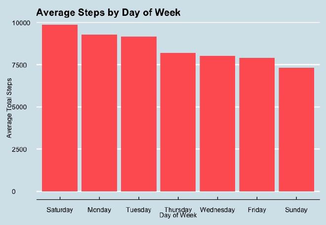
> sort(weekday_summary[, 1], decreasing = TRUE) # Total Steps Average
 Saturday    Monday   Tuesday  Thursday Wednesday    Friday    Sunday
 9871.123  9273.217  9182.692  8183.516  8022.864  7901.404  7297.855
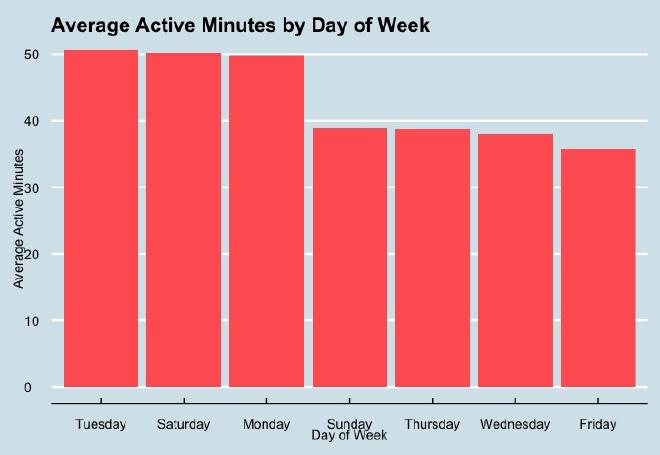
> sort(weekday_summary[, 2], decreasing = TRUE) # Active Minutes Average
  Tuesday  Saturday    Monday    Sunday  Thursday Wednesday    Friday
 50.66154  50.28070  49.80435  38.90909  38.71875  38.07576  35.73684
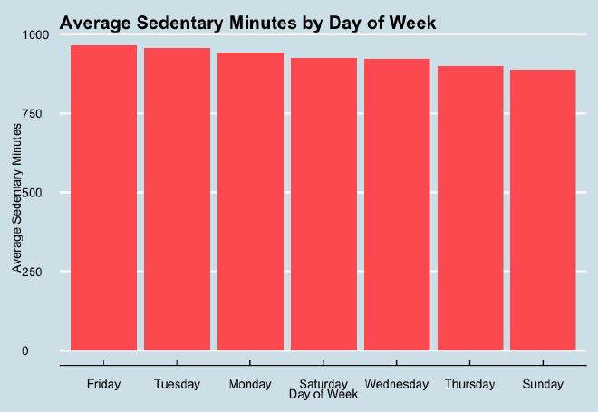
> sort(weekday_summary[, 3], decreasing = TRUE) # Sedentary Minutes Average
   Friday   Tuesday    Monday  Saturday Wednesday  Thursday    Sunday
 965.7719  956.6308  940.7826  927.2105  922.4242  901.3125  887.6727
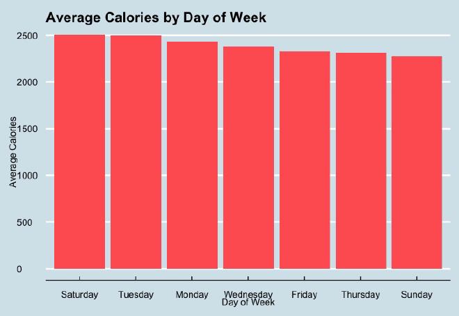
> sort(weekday_summary[, 4], decreasing = TRUE) # Calories Average
 Saturday   Tuesday    Monday Wednesday    Friday  Thursday    Sunday
 2506.895  2496.200  2431.978  2378.242  2329.649  2306.672  2276.600
> sort(weekday_summary[, 5], decreasing = TRUE) # Total Hours Asleep
   Sunday Wednesday    Monday  Saturday    Friday   Tuesday  Thursday
 7.545758  7.244697  6.991667  6.984503  6.757018  6.742308  6.688281
Using ggplot, I made several charts describing my findings:
weekday_summary1 <- as.data.frame(weekday_summary)

library(ggthemes)

# Average Steps Chart
ggplot(data = weekday_summary1, aes(x = reorder(as.character(row.names(weekday_summary1)), -Total_Steps_Ave), y = Total_Steps_Ave)) +
  geom_bar(stat="identity", fill = "#ff6262") +
  labs(title="Average Steps by Day of Week", x = "Day of Week", y = "Average Total Steps") +
  theme_economist()
# Active Minutes Average Chart
ggplot(data = weekday_summary1, aes(x = reorder(as.character(row.names(weekday_summary1)), -Active_Minutes_Ave), y = Active_Minutes_Ave)) +
  geom_bar(stat="identity", fill = "#ff6262") +
  labs(title="Average Active Minutes by Day of Week", x = "Day of Week", y = "Average Active Minutes") +
  theme_economist()
# Sedentary Minutes Average Chart
ggplot(data = weekday_summary1, aes(x = reorder(as.character(row.names(weekday_summary1)), -Sedentary_Minutes_Ave), y = Sedentary_Minutes_Ave)) +
  geom_bar(stat="identity", fill = "#ff6262") +
  labs(title="Average Sedentary Minutes by Day of Week", x = "Day of Week", y = "Average Sedentary Minutes") +
  theme_economist()
# Calories Average Chart
ggplot(data = weekday_summary1, aes(x = reorder(as.character(row.names(weekday_summary1)), -Calories_Ave), y = Calories_Ave)) +
  geom_bar(stat="identity", fill = "#ff6262") +
  labs(title="Average Calories by Day of Week", x = "Day of Week", y = "Average Calories") +
  theme_economist()
# Sleep Hours Average Chart
ggplot(data = weekday_summary1, aes(x = reorder(as.character(row.names(weekday_summary1)), -Total_Steps_Ave), y = Total_Steps_Ave)) +
  geom_bar(stat="identity", fill = "#ff6262") +
  labs(title="Average Hours of Sleep by Day of Week", x = "Day of Week", y = "Average Hours of Sleep") +
  theme_economist()
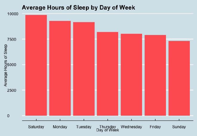
Interesting how both Tuesday and Monday are in the top three in each chart, even Average Sedentary Minutes. It seems that people are more likely to go easy on Fridays and stay up later. Overall, the differences between the days of the week aren’t as large as one might expect, but these differences are still notable enough to consider.
Hourly Data Analysis #
I imported hourlyMerged.csv into RStudio, where I could compare the relationship between calories, steps, and intensity. I first divided the activity hour column into activityDate and time, then converted them to the appropriate data types, then added times corresponding to the day of the week and the time of day:
library(lubridate)
hourlyMerged1$activityDate <- str_split_fixed(hourlyMerged1$activity_hour, " ", n = 2)[, 1]
hourlyMerged1$time <- str_split_fixed(hourlyMerged1$activity_hour, " ", n = 2)[, 2]
hourlyMerged1$activityDate <- as.Date(hourlyMerged1$activityDate, format="%Y-%m-%d")
hourlyMerged1$DayOfWeek <- format(as.Date(hourlyMerged1$activityDate), "%A")
breaks <- hour(hms("00:00:00", "05:59:59", "11:59:59", "17:59:59", "23:59:59"))
labels <- c("Night", "Morning", "Afternoon", "Evening")
hourlyMerged1$time  <- as.POSIXct(hourlyMerged1$time, format = "%H:%M:%S")
hourlyMerged1$TimeOfDay <- cut(x = hour(hourlyMerged1$time), breaks = breaks, labels = labels, include.lowest=TRUE)
colSums(is.na(hourlyMerged1)) # No NA values.
There appeared to be no strong correlation between intensity and either steps or calories burned:
> cor.test(hourlyMerged1$average_intensity, hourlyMerged1$Calories, method = "pearson")

    Pearson's product-moment correlation

data:  hourlyMerged1$average_intensity and hourlyMerged1$Calories
t = 147.75, df = 15393211, p-value < 2.2e-16
alternative hypothesis: true correlation is not equal to 0
95 percent confidence interval:
 0.03713366 0.03813135
sample estimates:
       cor
0.03763252

> cor.test(hourlyMerged1$total_intensity, hourlyMerged1$Calories, method = "pearson")

    Pearson's product-moment correlation

data:  hourlyMerged1$total_intensity and hourlyMerged1$Calories
t = 147.75, df = 15393211, p-value < 2.2e-16
alternative hypothesis: true correlation is not equal to 0
95 percent confidence interval:
 0.03713366 0.03813136
sample estimates:
       cor
0.03763252

> cor.test(hourlyMerged1$total_intensity, hourlyMerged1$step_total, method = "pearson")

    Pearson's product-moment correlation

data:  hourlyMerged1$total_intensity and hourlyMerged1$step_total
t = 170.87, df = 15393211, p-value < 2.2e-16
alternative hypothesis: true correlation is not equal to 0
95 percent confidence interval:
 0.04301144 0.04400866
sample estimates:
       cor
0.04351006

> cor.test(hourlyMerged1$average_intensity, hourlyMerged1$step_total, method = "pearson")

    Pearson's product-moment correlation

data:  hourlyMerged1$average_intensity and hourlyMerged1$step_total
t = 170.87, df = 15393211, p-value < 2.2e-16
alternative hypothesis: true correlation is not equal to 0
95 percent confidence interval:
 0.04301144 0.04400866
sample estimates:
       cor
0.04351006
In this case, I thought it might be worth analyzing what time of day participants were most active: night, morning, afternoon, and evening.
> hourMorning <- hourlyMerged1 %>%
+   filter(hourlyMerged1$TimeOfDay == "Morning") %>%
+   select(c(step_total, total_intensity, Calories))
>
> summary(hourMorning)
   step_total     total_intensity     Calories
 Min.   :   0.0   Min.   :  0.00   Min.   : 42.0
 1st Qu.:   0.0   1st Qu.:  0.00   1st Qu.: 68.0
 Median : 104.0   Median :  3.00   Median : 84.0
 Mean   : 374.8   Mean   : 12.06   Mean   :101.7
 3rd Qu.: 467.0   3rd Qu.: 16.00   3rd Qu.:117.0
 Max.   :8976.0   Max.   :180.00   Max.   :544.0
>
>
> hourAfternoon <- hourlyMerged1 %>%
+   filter(hourlyMerged1$TimeOfDay == "Afternoon") %>%
+   select(c(step_total, total_intensity, Calories))
>
> summary(hourAfternoon)
   step_total      total_intensity     Calories
 Min.   :    0.0   Min.   :  0.00   Min.   : 42.0
 1st Qu.:   37.0   1st Qu.:  0.00   1st Qu.: 77.0
 Median :  259.0   Median :  3.00   Median : 96.0
 Mean   :  519.6   Mean   : 12.06   Mean   :115.9
 3rd Qu.:  620.0   3rd Qu.: 16.00   3rd Qu.:131.0
 Max.   :10554.0   Max.   :180.00   Max.   :948.0
>
> hourEvening <- hourlyMerged1 %>%
+   filter(hourlyMerged1$TimeOfDay == "Evening") %>%
+   select(c(step_total, total_intensity, Calories))
>
> summary(hourEvening)
   step_total     total_intensity     Calories
 Min.   :   0.0   Min.   :  0.00   Min.   : 42.0
 1st Qu.:   0.0   1st Qu.:  0.00   1st Qu.: 69.0
 Median : 114.0   Median :  3.00   Median : 86.0
 Mean   : 370.9   Mean   : 12.06   Mean   :102.1
 3rd Qu.: 398.0   3rd Qu.: 16.00   3rd Qu.:113.0
 Max.   :8586.0   Max.   :180.00   Max.   :834.0
>
> hourNight <- hourlyMerged1 %>%
+   filter(hourlyMerged1$TimeOfDay == "Night") %>%
+   select(c(step_total, total_intensity, Calories))
>
> summary(hourNight)
   step_total      total_intensity     Calories
 Min.   :   0.00   Min.   :  0.00   Min.   : 42.00
 1st Qu.:   0.00   1st Qu.:  0.00   1st Qu.: 56.00
 Median :   0.00   Median :  3.00   Median : 68.00
 Mean   :  24.94   Mean   : 12.06   Mean   : 71.74
 3rd Qu.:   0.00   3rd Qu.: 16.00   3rd Qu.: 83.00
 Max.   :2844.00   Max.   :180.00   Max.   :669.00
I then put all the summaries together to get a better idea of what time of day people were most active:
> hour_Morn_list <-
+   list(
+     list("Total_Steps_Ave" = ~ mean(hourMorning$step_total)),
+     list("Calories_Ave" = ~ mean(hourMorning$Calories))
+   )
> hour_Morn_summary <- summary_table(hourMorning, hour_Morn_list)
> print.default(hour_Morn_summary)
                hourMorning (N = 3,886,786)
Total_Steps_Ave                    374.7585
Calories_Ave                       101.6646
attr(,"rgroups")
[1] 1 1
attr(,"n")
[1] 3886786
attr(,"class")
[1] "qwraps2_summary_table" "matrix"                "array"
>
> hour_Aft_list <-
+   list(
+     list("Total_Steps_Ave" = ~ mean(hourAfternoon$step_total)),
+     list("Calories_Ave" = ~ mean(hourAfternoon$Calories))
+   )
> hour_Aft_summary <- summary_table(hourAfternoon, hour_Aft_list)
> print.default(hour_Aft_summary)
                hourAfternoon (N = 3,825,364)
Total_Steps_Ave                      519.5996
Calories_Ave                         115.8662
attr(,"rgroups")
[1] 1 1
attr(,"n")
[1] 3825364
attr(,"class")
[1] "qwraps2_summary_table" "matrix"                "array"
>
> hour_Eve_list <-
+   list(
+     list("Total_Steps_Ave" = ~ mean(hourEvening$step_total)),
+     list("Calories_Ave" = ~ mean(hourEvening$Calories))
+   )
> hour_Eve_summary <- summary_table(hourEvening, hour_Eve_list)
> print.default(hour_Eve_summary)
                hourEvening (N = 3,784,154)
Total_Steps_Ave                    370.9224
Calories_Ave                       102.1464
attr(,"rgroups")
[1] 1 1
attr(,"n")
[1] 3784154
attr(,"class")
[1] "qwraps2_summary_table" "matrix"                "array"
>
> hour_Night_list <-
+   list(
+     list("Total_Steps_Ave" = ~ mean(hourNight$step_total)),
+     list("Calories_Ave" = ~ mean(hourNight$Calories))
+   )
> hour_Night_summary <- summary_table(hourNight, hour_Night_list)
> print.default(hour_Night_summary)
                hourNight (N = 3,896,909)
Total_Steps_Ave                  24.93547
Calories_Ave                     71.73854
attr(,"rgroups")
[1] 1 1
attr(,"n")
[1] 3896909
attr(,"class")
[1] "qwraps2_summary_table" "matrix"                "array"
> timeofday_summary_rows <- cbind(hour_Morn_summary, hour_Aft_summary, hour_Eve_summary, hour_Night_summary)
> timeofday_summary = t(timeofday_summary_rows)
>
> sort(timeofday_summary[, 1], decreasing = TRUE)
hourAfternoon (N = 3,825,364)   hourMorning (N = 3,886,786)   hourEvening (N = 3,784,154)
                    519.59962                     374.75847                     370.92242
    hourNight (N = 3,896,909)
                     24.93547

> sort(timeofday_summary[, 2], decreasing = TRUE)
hourAfternoon (N = 3,825,364)   hourEvening (N = 3,784,154)   hourMorning (N = 3,886,786)
                    115.86621                     102.14637                     101.66459
    hourNight (N = 3,896,909)
                     71.73854
Finally, let’s once again put those data into charts:
# Average Steps by Time of Day
ggplot(data = timeofday_summary1, aes(x = reorder(as.character(row.names(timeofday_summary1)), -Total_Steps_Ave), y = Total_Steps_Ave)) +
  geom_bar(stat="identity", fill = "#ff6262") +
  labs(title="Average Steps by Time of Day", x = "", y = "Average Total Steps") +
  theme_economist()

# Average Calories by Time of Day
ggplot(data = timeofday_summary1, aes(x = reorder(as.character(row.names(timeofday_summary1)), -Calories_Ave), y = Calories_Ave)) +
  geom_bar(stat="identity", fill = "#ff6262") +
  labs(title="Average Calories by Time of Day", x = "", y = "Average Calories") +
  theme_economist()
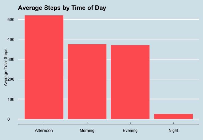
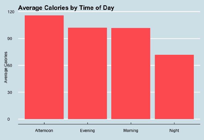
No surprise that nighttime ranks last for physical activity. People are slightly yet significantly more likely to be more active during the afternoon than the evening or morning.
Summary #
1. What are some trends in smart device usage? The clearest trend is that FitBit simply isn’t collecting enough data.
2. How could these trends apply to Bellabeat customers? If the customers can’t log this data easily, then they’re missing out on a lot of very useful insights.
3. How could these trends help influence Bellabeat marketing strategy? These gaps in FitBit’s data are a great opportunity for BellaBeat to step in and provide something their competitors have thus far been unable to provide.
Recommendations #
- Incentivize customers to engage with the app and device on “off days”.
- For example, if Friday is a day when customers are consistently less active and more sedentary, the app should encourage them to engage in some light physical activity.
- Investigate friction in the weight-logging feature.
- Body weight is important data for anyone trying to improve their health. Whatever is preventing customers from regularly logging their weight needs to be uncovered and corrected.
- Weight needs to be measured at regular intervals and under the same conditions for the data to be helpful. An individual’s weight can fluctuate dramatically throughout the day, so a person can appear to be up to ten pounds (4.5kg) heavier or lighter depending on when they logged their weight. This is one of the rare cases when too many readings can spoil the utility of the dataset. Perhaps the customer can be encouraged to set a weekly timer to remind them to weigh themselves under similar conditions. If they want to weigh themselves outside of these time frames, they should receive a dialog box confirming that they understand the issues with doing so.
- Perhaps there can be hardware integration with smart scales, much in the same way as BellaBeat’s Spring water bottle automatically tracks hydration.
- Encourage users to wear the device to bed.
- Sleep is just as important to a healthy life as exercise and a balanced diet. BellaBeat should strongly encourage their customers go to bed at an appropriate time for each of their schedules while wearing one of the company’s products. BellaBeat can really stand out in their field if they can use abundant and accurate sleep data to help their customers.
- It’s also possible that the particular device used to track sleep wasn’t conducive to tracking sleep. For example, maybe some customers find wearing a wristwatch to bed to be too uncomfortable to be worth it. In such a case, this might require a hardware solution.
- Improve data integration
- Even when the data has been gathered amply and correctly, they seem to be disconnected from each other. Sure, steps taken correlate strongly with calories burned, but that’s a banal observation. It’s very hard to see how someone can look at this FitBit data at a glance and use it to change their habits and routines. BellaBeat should not only be gathering better data than FitBit, but it should also leverage that data better to provide interesting and actionable insights to their customers.
- The customer should feel like their data is being gathered and deployed to improve their lives. This can incentivize them to more regularly log their data and wear the tracking devices while sleeping. Without this sense of purpose, the customer will stop engaging with the device seriously.
Acknowledgments #
I’d like to thank Ed Garcia for his guidance on how to divide the data into days of the week and times of the day.